Current account equilibria in EMs

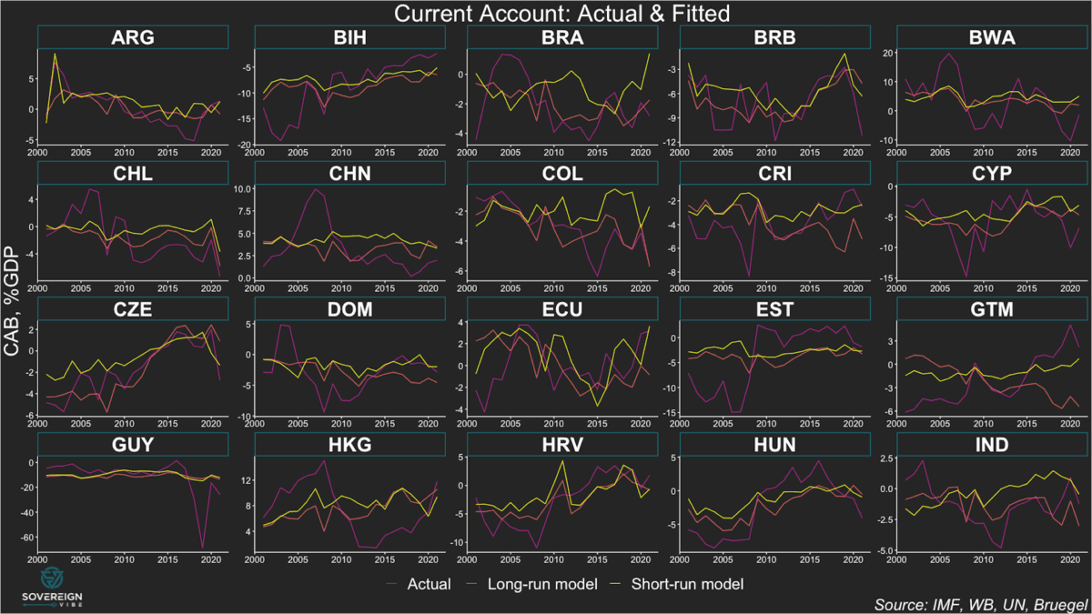
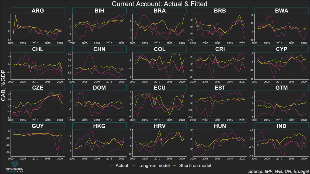
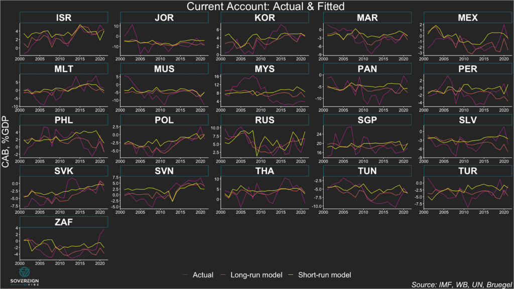
Following on from my estimates of current account equilibria in advanced economies, here I turn to emerging markets, which is after all the focus of this blog. I initially focused on AEs in an attempt to replicate as closely as possible an IMF empirical investigation of current account balances in this set of countries, as doing so is more methodologically prudent before expanding the analysis to EMs.

The goal of this work is to understand what a country’s current account balance should be (see my previous post for a breakdown of what CABs are), based on relevant characteristics as identified by the IMF in its model. These include the cyclically-adjusted government budget balances, demographic dependency ratios, and income level, which are all variables that tend to change only gradually over time. As such, they can be thought of as “long-term” variables, especially the latter two, which can be useful in trying to conceptualize where a country’s CAB ought to be.

In contrast, cyclical variables that are more volatile from year to year, such as real exchange rates, terms of trade, and domestic output gaps, as well as fiscal policy, theoretically should do a better job of predicting observed CAB readings. These can be thought of “short-term” variables, although I use the same fiscal variable in both the long- and short-run models.

The “long-run” model fitted values in these charts are the closest approximation I have now for current account equilibria in these EMs. But my confidence in these results is low and will require additional work, for the reasons described below.

Regretfully, I am far from satisfied with the results of this work so far, but have chosen to publish these interim conclusions in the interest of maintaining regular engagement with my audience. Worse still is that I had to exclude important EMs such as Indonesia from the analysis to maintain a balanced panel dataset, as data availability for some indicators didn’t go far back enough in time.

The good news is that both models have overall statistical significance and that each of the regressors in the short-run model is statistically significant.

Short-run model results

I’d still like to tweak the short-run model by adding a trade-weighted foreign output gaps as an independent variable and replacing the cyclically-adjusted budget indicator with a non-cyclically-adjusted budget variable. But, overall, I’m fairly content with the short-run model, as the fiscal, terms of trade, and real exchange rate regressors all behave as expected in relation to the CAB.

For methodological reasons, I dropped the lagged dependent variable that featured in the short-run AE model, which has decreased the R² readings in this short-run EM model, though I don’t see this as much of a problem.

Surprisingly, the domestic output gap is not negatively-related to the CAB but exhibits a positive, strong, and significant association. A positive output gap, meaning that economic growth is above-trend, often results in increased imports, thus placing downward pressure on the CAB. And this is indeed what I found in the short-run model for AEs: a negative, strong, and significant relationship.

Perhaps the reason behind the positive output gap-CAB relationship in EMs is to be found in exports as a common driver: strong exports could lead to a higher output gap and a higher CAB. Many EMs rely heavily on exports for economic growth, whether of manufactured goods, commodities, or services.

Short-run model variables

• Deviation from the in-sample average of the general government cyclically-adjusted budget balance adjusted for nonstructural elements beyond the economic cycle, as a share of potential GDP. Countries with higher-than average government budget balances should be able to attract larger portions of global current account surpluses. This is confirmed by the positive coefficient at 1% significance.
• Domestic output gap: actual output minus potential output in current USD (logarithmic difference). Economies in the boom phase of an economic cycle can experience strong import growth, appreciated exchange rates, and stronger remittance and primary income outflows, putting the current account under pressure. Unexpectedly, the coefficient is positive, and is also large and significant. Theoretically, exports could be a common driver of output gaps and CABs in EMs, as they are positively associated with both.
• One-year change in the terms of trade, i.e. the ratio of the price of exports to the price of imports. The coefficient is positive and significant, as expected.
• One-year change in the REER. The coefficient is negative and significant, as expected, because high REERs can lead to imports becoming relatively cheap, thus increasing import volumes, and lead to exports becoming relatively expensive, thus decreasing export volumes.

Regression Results – 41 Emerging Economies

	Dependent variable:
	Current Account Balance, %GDP
	panel	coefficient
	linear	test
	(1)	(2)
	random.shortrun	random.pcse.shortrun
sur_dev	0.439***	0.439***
	(0.056)	(0.065)
ogap_usd.logdiff	15.920***	15.920**
	(3.543)	(8.019)
tot_1d	0.061***	0.061***
	(0.022)	(0.022)
reer_1d	-0.072***	-0.072***
	(0.021)	(0.018)
Constant	-1.054	-1.054
	(0.735)	(1.022)
Observations	861
R2	0.097
Adjusted R2	0.093
F Statistic	92.337***
Note:	*p<0.1; **p<0.05; ***p<0.01

Long-run model results

As for the long-run model, alas only two of its four independent variables are statistically significant after controlling for heteroskedasticity and autocorrelation: the budget surplus indicator and the old-age dependency ratio.

The child-age dependency ratio and income level were both statistically insignificant, as was the case in the advanced economy model. As such, in further work on this I will be discarding these two regressors and replacing them with something related to private savings. Doing so would complement the public savings approach already captured by the budget variable.

Moreover, the adjusted-R² is laughably low in this model. While achieving a high R² isn’t the most important consideration in constructing a good model with unbiased, efficient estimators, I’d still like to see something higher.

One other area of improvement for this long-run CAB model would be to run the independent variables against underlying CABs – which have the cyclical impact of output gaps stripped out and real exchange rate effects worked in – rather than against observed, actual CABs.

Long-run model variables

• Deviation from the in-sample average of the general government cyclically-adjusted budget balance adjusted for nonstructural elements beyond the economic cycle, as a share of potential GDP. Countries with higher-than average government budget balances should be able to attract larger portions of global current account surpluses. This is confirmed by the positive coefficient at 1% significance.
• The deviation from the in-sample average of the child-age dependency ratio on the 20-64 year-old working-age population, i.e. people 19 and under. I tested this variable on the intuition that the child dependency ratio could well be negative, not only due to the income effect as noted by Faruqee and Isard, but also due to the large amounts of consumption (which pushes down savings, increases imports etc) associated with children’s parents at the height of their income generation, family activities, and the associated demographic profile that such countries might have. In this two-ways fixed effects model it is insignificant when standard errors are controlled for heteroskedasticity and autocorrelation. It is also unexpectedly positive.
• The deviation from the in-sample average of the old-age dependency ratio on the 20-64 year-old working-age population, i.e. people 65 and over. My intuition with this variable is that it would be positive because of the high level of savings that elderly people have, despite doubts as to the degree to which the elderly can generate positive savings flows for themselves. The sign was positive, as expected, a statistically significant.
• Deviation from the in-sample average of GNI per capita on a PPP basis, adjusted for the country’s output gap to equate the observation to what it would be if the economy were running at potential. Unexpectedly, the coefficient is negative: theoretically, greater availability of income and thus savings opportunities in wealthier countries should lead to a higher CAB. Yet this result is insignificant in the long-run model.

Regression Results – 41 Emerging Economies

	Dependent variable:
	Current Account Balance, %GDP
	panel	coefficient
	linear	test
	(1)	(2)
	fixed.twoways.longrun.b	fixed.twoways.hac.longrun.b
sur_dev	0.371***	0.371***
	(0.060)	(0.090)
dem_chd_dev	0.157***	0.157
	(0.051)	(0.119)
dem_old_dev	0.433***	0.433*
	(0.147)	(0.227)
ypcap_dev	-0.056	-0.056
	(0.039)	(0.114)
Observations	861
R2	0.106
Adjusted R2	0.035
F Statistic	23.716*** (df = 4; 796)
Note:	*p<0.1; **p<0.05; ***p<0.01