Current account equilibria in AEs

Have you ever wondered what a country’s current account balance should be? If you’re a macroeconomist or investor, then chances are that you have. While plenty has been written on how to measure “equilibrium” current account balances, to my knowledge there is precious little publicly-available information as to what these actually are. So I’ve drawn from the existing literature on the subject in an attempt to construct a model of where a country’s current account should stand over the medium-to-long term.

If you’re asking yourself why you should care about “normal” current account balances, first of all a quick refresher. The current account is the sum of a country’s goods and services trade balances (i.e. exports minus imports), its net primary income (e.g. wages and investment income from abroad), and net secondary income (i.e. grants from foreign donors and workers’ remittances from abroad). Adding consumption and investment to the current account is equal to gross national income, and some simple arithmetic shows that the CAB is also equivalent to savings minus investment:

CAB = PIB + SIB + X - M

GNI = PIB + SIB + X - M + C + I = CAB + C + I

CAB = GNI - C - I = S - I

From a savings minus investment perspective, the CAB is the sum of the public sector’s (i.e. government) S - I balance, which is closely related to the government’s budget, and the private sector’s S - I balance. Surplus current account flows lead to the accumulation of foreign currency reserves and/or net foreign assets acquisition, while a deficit must be financed by capital from abroad and/or the depletion of the central bank’s foreign currency reserves.

Exchange rates

Exchange rates obviously play a pivotal role in influencing a CAB, which is why “currency wars” periodically erupt, with nations accusing each other – sometimes with good reason – of artificially devaluing their currencies in order to boost their CABs. Currencies are also one of the main reasons to take an interest in CABs, because the latter help measure whether a currency is over- or undervalued.

Focusing on a country’s real effective exchange rate, i.e. its trade-weighted exchange rate incorporating relative price levels of its trading partners, there are multiple approaches to assessing REER fair value, one of which involves measuring cyclically-adjusted (i.e. “underlying”) current account deviations from the equilibrium current account:

REER deviation from FV ≈ CABunderlying - CABequilibrium

Undervalued currency: CABunderlying > CABequilibrium

Overvalued currency: CABunderlying < CABequilibrium

CAB modeling results

The first step in this analysis is to measure equilibria CABs that reflect a country’s non-cyclical characteristics over the medium-to-long run, hewing closely to past work on the subject, including by analyzing the same group of 21 advanced economies. I’ve developed two models in order to track these CABs: short-run estimates of observed CAB readings and a long-run framework to approximate equilibria CABs.

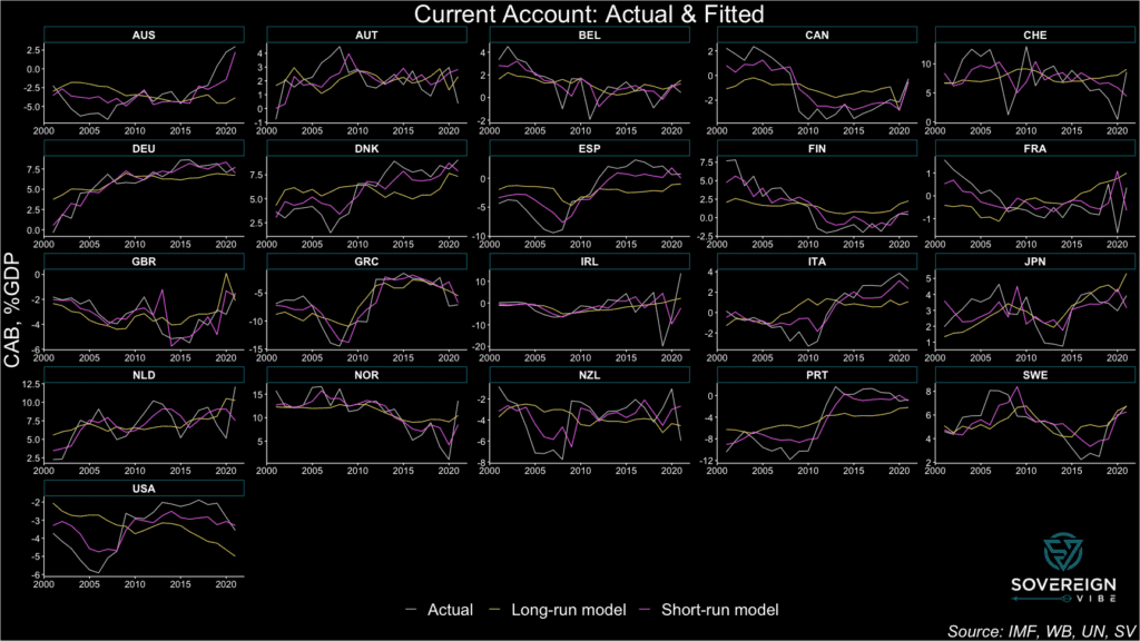
The results are presented in the chart below, featuring CAB observations, the long-run model, and short-run model. The latter tracks the actual CAB results relatively closely, in large part because the cyclical/short-term variables exhibit high degrees of statistical significance in the model. Moreover, the observed CAB values are obviously driven by cyclical factors in addition to long-term trends.

In contrast, the long-run model has much lower explanatory power compared to the short-run model with respect to minimizing residual deviations away from the observed CABs. But this is precisely the point. Medium- to long-run CAB equilibria should be relatively stable compared to the cyclical volatility exhibited by the actual CABs and their short-run fitted values.

Still, the long-run model estimates of CAB equilibria are subject to a high degree of uncertainty, given the the presence of statistical significance in only one of the three independent variables and low adjusted R² (see regressions below).

Model & variable selection

The analysis uses panel data for 21 advanced economies from 2001 – 2021 and included various statistical tests for selecting appropriate models and controlling for heteroskedasticity, serial correlation, cross-sectional dependence, and stationarity. For both the short- and long-run approaches, fixed effects models were chosen over OLS or random effects. Only individual (i.e. country) fixed effects were included; time-fixed effects were unnecessary.

The current account balance as a percentage of nominal GDP served as the dependent variable for both the short- and long-run frameworks.

Short-run model variables

• One-year lag of the dependent variable, i.e. the current account / GDP ratio. The high degree of inertia in CAB time series processes resulted in a large positive coefficient at a high degree of significance.
• Deviation from the in-sample average of the general government cyclically-adjusted budget balance adjusted for nonstructural elements beyond the economic cycle, as a share of potential GDP. Countries with higher-than average government budget balances should be able to attract larger portions of global current account surpluses. This is confirmed by the positive coefficient at 1% significance.
• Deviation from the in-sample average of GNI per capita on a PPP basis, adjusted for the country’s output gap to equate the observation to what it would be if the economy were running at potential. As expected, the coefficient is positive – reflecting the CAB-GNI conceptual overlap, greater availability of income and thus savings opportunities to wealthier countries, and the need for capital deepening in less developed countries. It is significant when standard errors are adjusted for heteroskedasticity and autocorrelation in this fixed effects model.
• Domestic output gap: actual output minus potential output in current USD (logarithmic difference). Economies in the boom phase of an economic cycle can experience strong import growth, appreciated exchange rates, and stronger remittance and primary income outflows, putting the current account under pressure. As expected, the coefficient is negative, large, and significant.
• One-year change in the terms of trade, i.e. the ratio of the price of exports to the price of imports. The coefficient is positive and significant, as expected.
• One-year change in the REER. The coefficient is negative and significant, as expected, because high REERs can lead to imports becoming relatively cheap, thus increasing import volumes, and lead to exports becoming relatively expensive, thus decreasing export volumes.

Regression Results – 21 Advanced Economies

	Dependent variable:
	Current Account Balance, %GDP
	panel	coefficient
	linear	test
	(1)	(2)
	fixed.shortrun	fixed.hac.shortrun
cab.t_1	0.582***	0.582***
	(0.040)	(0.125)
sur_dev	0.221***	0.221**
	(0.052)	(0.089)
ypcap_dev	0.026	0.026**
	(0.018)	(0.011)
ogap_usd.logdiff	-6.593*	-6.593*
	(3.994)	(3.620)
tot_1d	0.091***	0.091**
	(0.021)	(0.044)
reer_1d	-0.050*	-0.050**
	(0.028)	(0.024)
Observations	441
R2	0.456
Adjusted R2	0.422
F Statistic	57.907*** (df = 6; 414)
Note:	*p<0.1; **p<0.05; ***p<0.01

Long-run model variables

• Deviation from the in-sample average of the general government cyclically-adjusted budget balance adjusted for nonstructural elements beyond the economic cycle, as a share of potential GDP. Countries with higher-than average government budget balances should be able to attract larger portions of global current account surpluses. This is confirmed by the positive coefficient at 1% significance.
• The deviation from the in-sample average of total dependency ratio of non-workers on the 20-64 year-old working-age population, i.e. people 19 and under & 65 and over. Faruqee and Isard contend that the dependency ratio should be negatively associated with current account equilibria, partly due to the income effect, and find it to be so in their 1970s – 1990s data. Here the sign is positive, somewhat unexpectedly, and is statistically insignificant.
• The deviation from the in-sample average of the child-age dependency ratio on the 20-64 year-old working-age population, i.e. people 19 and under. I tested this variable on the intuition that the child dependency ratio could well be negative, not only due to the income effect as noted by Faruqee and Isard, but also due to the large amounts of consumption (which pushes down savings, increases imports etc) associated with children’s parents at the height of their income generation, family activities, and the associated demographic profile that such countries might have. Although this relationship showed up as negative in OLS, in this fixed effects model it is insignificant and unexpectedly positive.
• The deviation from the in-sample average of the old-age dependency ratio on the 20-64 year-old working-age population, i.e. people 65 and over. My intuition with this variable is that it would be positive because of the high level of savings that elderly people have, despite doubts as to the degree to which the elderly can generate positive savings flows for themselves. The sign was positive, as expected, but small and insignificant.
• Deviation from the in-sample average of GNI per capita on a PPP basis, adjusted for the country’s output gap to equate the observation to what it would be if the economy were running at potential. As expected, the coefficient is positive – reflecting the CAB-GNI conceptual overlap, greater availability of income and thus savings opportunities to wealthier countries, and the need for capital deepening in less developed countries. Yet this result is weak and insignificant in the long-run model.

Regression Results – 21 Advanced Economies

	Dependent variable:
	Current Account Balance, %GDP		cab_ngdp
	panel	coefficient	panel	coefficient
	linear	test	linear	test
	(1)	(2)	(3)	(4)
	fixed.longrun.a	fixed.hac.longrun.a	fixed.longrun.b	fixed.hac.longrun.b
sur_dev	0.481***	0.481***	0.478***	0.478***
	(0.062)	(0.125)	(0.062)	(0.129)
dem_tot_dev	0.086	0.086
	(0.067)	(0.134)
dem_chd_dev			0.173	0.173
			(0.143)	(0.361)
dem_old_dev			0.048	0.048
			(0.087)	(0.162)
ypcap_dev	0.014	0.014	0.012	0.012
	(0.023)	(0.035)	(0.023)	(0.038)
Observations	441		441
R2	0.148		0.149
Adjusted R2	0.101		0.100
F Statistic	24.141*** (df = 3; 417)		18.201*** (df = 4; 416)
Note:	*p<0.1; **p<0.05; ***p<0.01