Categories
Geopolitics

Senegalese exceptionalism, for now 🇸🇳

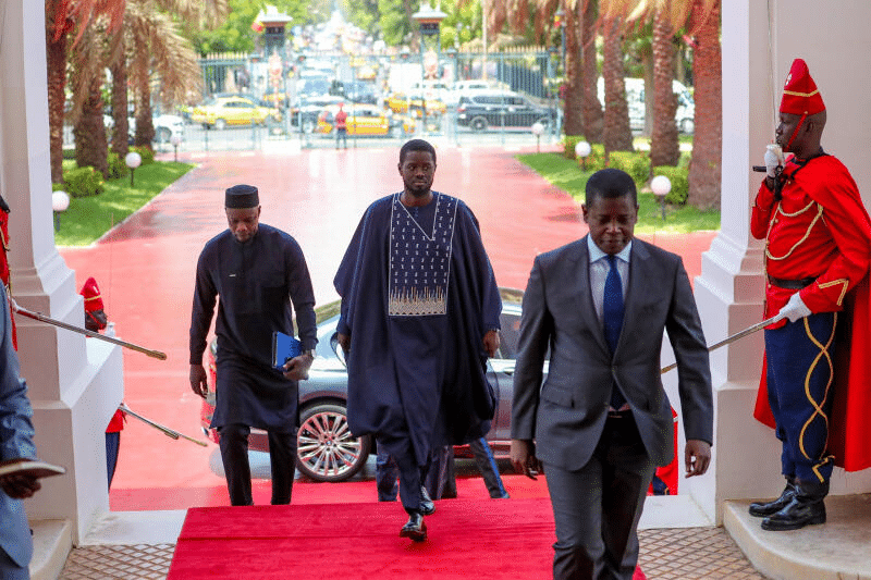
Today’s spotlight is on Senegal’s presidential election in March 2024 and the spectacular rise to power of political novice Bassirou “Diomaye” Faye, a 44-year old former tax inspector who went from prison to the presidency in scarcely 10 days. Digging beneath the surface of the electoral results reveals some oft-neglected ethnic undercurrents at play in Senegal and elsewhere in the Sahel that investors and observers should keep front of mind.

Why democratic stability is so rare in the Sahel

One of the things that struck me when living and working in Africa was the yawning gap between the international press coverage of electoral politics and the realities on the ground, which were both obvious and patiently explained to me by local friends.

I am of course referring to the ethnic dimensions of politics that are ever-present in so many African countries but that mainstream international media so often ignores.

In Africa, ethnicity doesn’t explain everything, but nothing can be explained without ethnicity.

Bernard Lugan

Democracy wins

Last month’s presidential elections in Senegal were first and foremost about the Senegalese people expressing their desire for change. As things currently stand, it is also a positive story of the country’s institutions resisting to pressure.

Indeed, Senegal has come back from the brink, after outgoing president Macky Sall sought to delay the elections indefinitely, and which – thankfully – the Constitutional Council overruled. The vote on 24 March saw opposition candidate Bassirou “Diomaye” Faye win a resounding victory that precluded the need for a second round runoff. A former tax inspector and political novice, Faye had been released from politically-motivated imprisonment only days before.

Source: Senegal’s Presidential Office, via Reuters & Le Monde

Yet the triumph was above all for Senegalese democracy, with government candidate Amadou Ba conceding the next day. The country thus remains a beacon of democratic stability with peaceful transitions of power since independence in an otherwise fragile region that has recently suffered a wave of coups d’état: Mali, Burkina Faso, Niger, Guinea. Beyond West Africa, Sudan, Chad, and Gabon have each had recent, idiosyncratic, coup-like political instability as well.

Mapping the ethnic X factor

I don’t want to exaggerate the importance of ethnicity in this election. For all intents and purposes, the result is a clear repudiation of Sall’s government and his anointed would-be successor, Ba, and overrides potential ethnic considerations.

Nevertheless, comparing a map of the electoral results to an ethno-linguistic map of Senegal suggests that ethnicity is still important. Sall is Fula (in French: Peul) and has had his political stronghold in the northern parts of the country, where many Fula live. These voting patterns were borne out in March’s election, with Ba getting much of his support from Fula-populated areas.

Source: Wikipedia
Source: G.G. Beslier, Le Sénégal

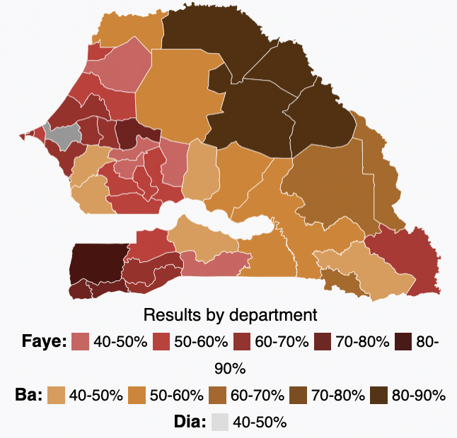
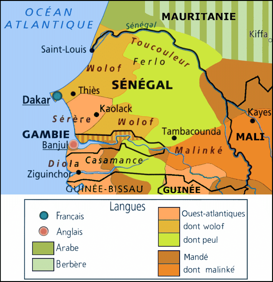
In contrast, Faye was much more dominant in areas populated by the Wolof, the Mandé / Malinké in the southeast and south, and in the southwest. Faye was until recently the right-hand man of Ousmane Sonko, who was ultimately prevented from running in the election. Sonko hails from the southwestern city Ziguinchor, where Faye secured a strong turnout, and has been chosen as prime minister.

The Sahelian ethno-democratic-demographic doom loop

On a continent that crams some 3000 ethnic groups speaking around 2100 languages into a mere 54 countries, it is myopic to completely ignore the ethnic undercurrents at play, even in cases where it isn’t the primary driver. Yet analyzing the political salience of ethnicity in Africa is more than just a useful intellectual exercise.

Think how, for example, as the largest nomadic pastoral community in the world, the Fula are present in Senegal and Guinea, and in Chad and Cameroon, and in every country in between. As climate change drives the Sahara’s expansion ever southward through the Sahel, we can expect land use-driven tensions to continue rising between the more martially-oriented nomadic pastoralists of the north and the more numerous sedentary agriculturalists to the south.

To that point on demographics, Western democratic ideals imposed on an African context partly explains many countries’ breakneck population growth. Individualism is at the center of the one-person one-vote approach to electoral democracy and works well in many parts of the world. But traditions of individual liberty were only introduced to African countries recently, where, historically, communitarian-led structures of societal organization tended to dominate.

Senegal’s population is growing at a rapid clip.

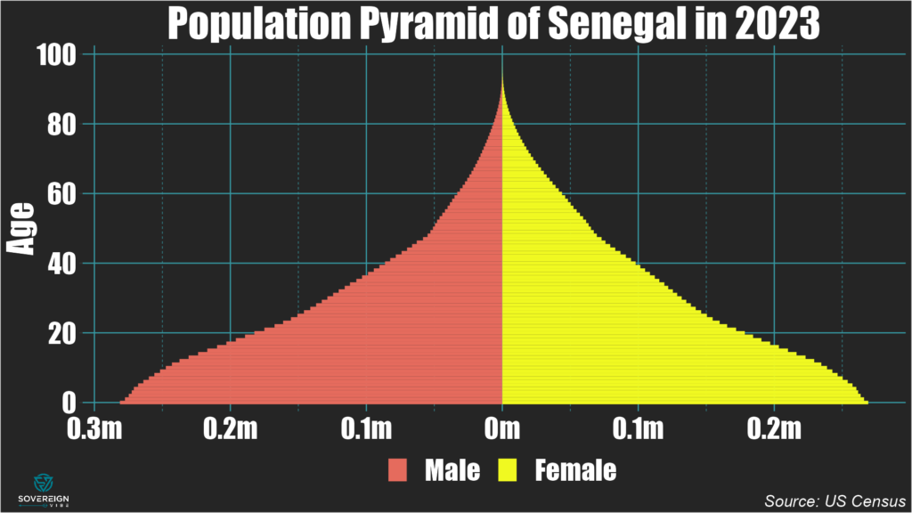
Thus Western-style democracy has incentivized each ethnic group to vie for political power by growing its population. This makes complete sense if one recognizes the communitarian focus that continues to drive politics in so many African countries to this day. Case in point, as of 2023 Senegalese women give birth to four children on average, and 75% of the country’s population is under 35 years old. Of course, the usual caveat applies: no single factor is fully responsible for a demographic outcome.

The bitter irony is that democracy has destabilized several of Senegal’s neighbors precisely because it has inverted the power relationship between the previously-dominant nomads and the sedentary farmers. Historically, these fierce warrior-pastoralists didn’t really require strength in numbers to subjugate their more pacific southern neighbors.

But in a context where democracy excludes the nomads from political power, it should not be at all surprising that these peoples would try to revolt or secede. This is precisely the driving force behind the ongoing conflicts and instability across the near-entirety of the Sahelian arc, rather than some inchoate jihadism. The several Tuareg / Azawad rebellions that have occurred since the 1960s serve as a prime example. Senegal alone has been spared. For now.

With all that in mind, can a victory of democracy in an African context be anything other than a pyrrhic one? I certainly hope so, and Senegal’s institutions give good reason to. Yet even as this result is rightly celebrated, the specter of roiling demographics and instability throughout so much of the region looms large over West Africa’s future.

What next for investors?

Investors have so far reacted to Faye’s victory with caution, as he is in many ways an unknown entity. It is still early days, so investors ought to remain circumspect while waiting to see the shape that his economic policies end up taking.

For now, what we know from Faye’s inauguration is that the economic agenda will focus on reducing cost-of-living pressures and on tackling corruption, while also having to address the high unemployment rate in this youthful country. On the external front, Faye and Sonko have espoused sovereignty and deep change, including reforms to or a complete transition away from the CFA currency.

Abandoning the CFA could prove tricky, as the currency has been a source of stability throughout much of the region, aside from a sharp devaluation in 1994. On the other hand, Senegal likely has the policy credibility and institutional strength to pull it off. Moreover, the CFA is almost certainly highly overvalued, so the move to a more flexible currency could benefit export activity.

The French Connection

As for the relationship with France, Sall had kept close ties while also diversifying Senegal’s partners. It seems likely that Faye will keep Paris at arm’s length, without necessarily shutting the door entirely, if the cordial 30-minute conversation he had with Macron last week is anything to go by.

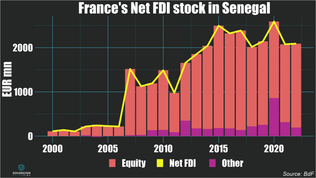
In the meantime, France’s net foreign direct investment stock in Senegal has remained above the €2bn mark in recent years, unlike declines in the French economic presence that have been registered elsewhere in francophone Africa. This level of FDI involvement in Senegal is close to 8% of GDP and represents nearly a fifth of FDI in the country, underscoring the ongoing presence that French economic interests are likely to have.

Categories
De-dollarization

Rise of the yuan? Not so fast

Berkeley-based economist and titan of the profession Barry Eichengreen notes that the dollar’s reserve currency status is continuing to erode in favor of “non-traditional reserve currencies”. But looking closely at the same recently-released IMF data through Q4 2023 paints a more nuanced picture.

At end-2016, the IMF reclassified yuan holdings from “other” to its own explicit category, so I’ve calculated cumulative changes from Q1 2017 onwards:

  • While the USD’s share in international reserves holdings have dropped by about 7 percentage points since then…
  • …the biggest beneficiary is neither the yuan nor “other” currencies…
  • …but in fact the yen.
  • The yuan has increased its share by about 1 percentage point…
  • …but the euro, pound, and Australian & Canadian dollars have seen their shares increase as well, for a combined total of over 2 percentage points.

So the shift away from the dollar is just as much – if not more – about a rotation into G7+ currencies as it is towards the yuan and other non-traditional reserve currencies. I’ve written previously about how a sizable chunk of Russia’s reserves have been held in Japan and how GBP, AUD, and CAD have been eating up some of the USD’s share.

Categories
De-dollarization

On the hunt for Russia’s reserves

When it comes to appropriating Russia’s central bank reserves for supporting Ukraine, some influential Western constituencies seem to think that the G7 leadership can and should dish out punishment without considering trifling matters such as due process. Such has been the Western enthusiasm for championing the Ukrainian cause, that they might have been right about this – or at least they were until recently. Also, where in the world are the Bank of Russia’s frozen assets?

Back in 2022, some of the many sanctions that several Western countries imposed on Russia in response to its invasion of Ukraine ended up freezing a lot of Russian assets held in various jurisdictions. The Bank of Russia’s immobilized reserves stand somewhere in the $300-350bn range, though it’s not quite clear where exactly it is all held. The quantum rises further, to around $400bn, if one includes the $58bn of Russian billionaire money also currently under sanctions.

That’s a lot of cash, obviously: Ukraine’s nominal GDP is only about $160bn, after having dropped by a third in 2022. With much of Ukraine’s economy and infrastructure in ruins and amid some setbacks on the battlefield, calls for repurposing Russia’s reserves to support and rebuild Ukraine have gained traction in recent months.

Location, location, location

As with so many other examples of opacity plaguing the international financial architecture, it’s unclear where exactly all of the Bank of Russia’s frozen assets actually are. Location matters because it will have at least some bearing as to how any appropriation gets carried out.

The little we know

The chart below is based on a G7 finance ministers’ statement in October 2023 and information posted on Switzerland’s government website in May 2023. The total in the chart comes out to just under $290bn, using current exchange rates, with the Belgian central securities depository Euroclear holding the lion’s share.

Amid reports of $300-$350bn in immobilized Russian central bank reserves, it’s hard to tell where those other $10-60bn in assets might be – or if those numbers are just entirely made up.

Even the “identified” locations in the chart are ambiguous, with the “EU – Other” and “G7 – Other” categories accounting for nearly $80bn.

Detective work

It turns out I’m not the first person to be puzzled by the mysterious whereabouts of Russia’s frozen assets. Nor the second, nor the third.

Inspiring myself from those who came before, I’ve taken a look at BIS data on banks’ liabilities to residents of Russia. Generally speaking, these seem to usually be in the form of deposits owned by entities and persons residing in Russia.

And sure enough, some of those massive Euroclear deposits show up in the chart above, around $136bn. This is less than the $196bn identified by the G7 statement, presented in the pie chart on immobilized reserves, meaning that the difference is presumably because $60bn of the assets aren’t bank liabilities (or simply weren’t reported to the BIS).

The amount of bank liabilities to Russia located in Switzerland are of a similar amount to the ~$8bn in Bank of Russia reserves that the Swiss authorities have reported sanctioning. As with Belgium, this suggests at least partial overlap.

As for the “Other EU” category representing $22.9bn in the first chart, France looks like the primary EU location based on its sizable cross-border bank liabilities to Russia. Press reports appear to confirm this – and that Germany also has Bank of Russia assets.

But it’s still unclear where those $55.5 bn in “Other G7” are held, though there aren’t too many suspects.

Pre-war breakdown

It shouldn’t really come as a surprise that the Bank of Russia has stopped publishing some of its statistics since the war escalated in 2022. But it sure makes it harder – or downright impossible – to know where its international reserves are located.

The last publicly-available data point is from June 30, 2021 and comes from the bank’s last Foreign Exchange and Gold Asset Management Report, released in 2022. Multiplying the $585.3bn total by the published percentages yields the following breakdown in the chart below:

The total held in G7 (i.e. sanctioning) countries – Austria, Canada, France, Germany, Japan, UK, USA – sums to $284.4bn, which is roughly equal to the G7’s October 2023 statement.

Two things:

  • First of all, France held the largest slice of any EU country at the time. Although Germany had a sizable chunk as well, this reconfirms France as the leading candidate for “Other EU.”
  • Secondly, the $58.5bn of Bank of Russia reserves held in Japan in 2021 corresponds neatly to the $55.5bn in “Other G7” in the first chart, which is about as clear an answer as I can hope to glean.

To seize or not to seize?

On the face of it, the arguments for appropriating the reserves make good sense. Ukraine currently requires around $100bn of support annually, $40bn of which is for balance of payments and budgetary purposes and $60bn for the military. Moreover, estimated damage to Ukraine amounts to ~$650bn.

These are steep bills, to say the least, and Kyiv really needs all the money it can get. So, rather than having Western and Ukrainian taxpayers, and Ukraine’s creditors, foot the entire bill, using Russian money amounts to fair burden-sharing, or so the argument goes.

A poisoned chalice

Although there is a strong case for using Russian assets to help Ukraine, the counterargument is also valid. Seizing the assets could set a negative precedent and lead to further global fragmentation, in a world that is already suffering from the effects of deglobalization.

Ambivalence towards Ukraine in much of the non-Western world suggests that appropriating the Bank of Russia’s reserves would be poorly-received and erode trust in Western institutions and the international rules-based order. Worse still, doing so without a solid legal basis could backfire spectacularly in the court of global public opinion.

The irony is that the West would be perceived to be stealing from a regime that it itself views as a kleptocracy. Given their immense wealth, G7 member countries are not condemned to use the weapons of their Russian opponents against them. Despite budgetary pressures, inflation, and other economic challenges, US support for Ukraine pales in comparison to spending on past wars, indicating room for more support.

Outright appropriation could be a major win for the Kremlin, especially if done without a strong legal foundation, without really inflicting further damage on Russia since the reserves are already immobilized. Putin could use it as evidence of Western moral bankruptcy and institutional hypocrisy in outreach to receptive audiences in the Global South. Moscow’s kleptocrats would likely be gleefully rubbing their hands at a new excuse for expropriating any remaining Western businesses in the country.

Furthermore, in the case of seizure, it is unclear if any Western businesses, e.g. Danone, Carlsberg, will have a claim to compensation for their lost assets in Russia, or if all the money would end up going to support Ukraine.

Deep freeze

There are of course other intermediate solutions. The least controversial one is to send the €4.4bn in interest income earned by Euroclear in 2023 – and which belongs to Euroclear – on its sanctioned Russian assets to Ukraine. Another policy proposal is to use the assets as collateral for bonds, whose proceeds would be directed to Ukraine, though France and Germany – as well as the Euroclear CEO – have come out against it.

The most likely outcome seems to be that the assets remain frozen for the foreseeable future while Western policymakers find whether or not there is a path forward. There may not be, for the simple reason that Europe is reticent.

If Donald Trump returns to the White House next January, the prospects of collateralization or seizure would be even more remote. Even now, the Republican party has already abandoned its erstwhile fervor for the Ukrainian cause, holding up a $60bn aid package for Ukraine in Congress.

It’s all so unfortunate because Ukraine desperately needs support, including a Marshall Plan to rebuild. But the truth is that it needed a Marshall Plan 30 years ago, as did Russia and all the other post-Soviet republics.

By failing to help rebuild the post-Soviet space then, the West missed a unique chance to help foster stability in this part of the world and at a much lower cost – especially in blood but also in treasure. As a result, the price to pay is much higher today, whether or not Ukraine ends up getting Russia’s assets.

Categories
Macro

Fair value exchange rates in EM Asia

  • FX fair value estimates for eight EM Asia economies point to more over- rather than under-valuation across the region…
  • …so the real depreciations registered by most of the region’s currencies last year has pushed many (but not all) towards fair value.
  • Inflation differentials are now playing a larger role in determining REERs compared to the pre-pandemic era.

Currencies in emerging markets Asia mostly declined in real terms in 2023. Pakistan registered the sharpest real exchange rate depreciation, though China also weakened significantly on the back of much less inflationary pressure in the country relative to its trading partners.

REER trends in EM Asia

Of the eight EM Asia countries covered below, only the Philippine peso and Korean won strengthened in real terms in 2023, though the Singaporean and (possibly) Hong Kong dollars were also in positive territory for the year.

For each country, I provide a chart that breaks down the contributions of to the real exchange rate:

  • The nominal effective exchange rate: Remember that “effective” implies a trade-weighted calculation against all trading partner currencies.
  • Inflation differentials: This indicator looks at the month-on-month changes of the ratio of the domestic country’s consumer price index versus the trade-weighted CPIs of its trading partners. A positive (negative) differential means that the domestic country is experiencing higher (lower) inflation than its trading partners are.

As for fair values, those are covered in the next section of this post.

🇨🇳 China: The yuan depreciated by around 7.5% in real terms in 2023, on the back of two years of mild appreciation. Despite some nominal weakening, it is mostly inflation differentials driving the real depreciation, as deflationary pressures in the Middle Kingdom stand in marked contrast to the rising prices experienced by its trading partners in recent years.

🇮🇳 India: The rupee experienced a real depreciation of about 3% in 2023 against its trading partners. Comparatively low inflation and some nominal currency weakening in H2 were both at play.

🇵🇰 Pakistan: The rupee declined by around 8% in real terms in 2023, following a smaller drop the previous year. The decrease in nominal effective terms was even larger, as inflation in Pakistan was higher than that of its trading partners for the entire year.

This content is for members only.

Categories
Geopolitics

Ukraine: two, ten, or thirty years on?

Today marks the grim anniversary of Russia’s full-scale invasion of Ukraine on February 24, 2022. Yet the conflict since 2022 is in many ways larger than the current military operations on the ground, both in terms of time and space. It is of course only the latest and most intense iteration of Russian aggression in the country, which started in earnest in 2014 with Russia seizing Crimea and launching military operations in the Donbas under the pretext of supposed separatism.

Spatially, events in Ukraine have global implications for geopolitical competition between the West and Russia, along with its allies of convenience – chief among them China but also pariahs such as North Korea and Iran. In tandem with the Covid-19 pandemic, the 2022 war in Ukraine marks the end of an era: the second of two death knells of the post-Cold War period.

Macroeconomic snapshot

Beyond the immense human toll, social disruption, and infrastructure destruction, the macroeconomic effects on Ukraine since 2022 have also been tremendous, obviously. The budget deficit went from a respectable -3.7% of GDP in 2021 to a gaping hole of nearly -30% in 2022, and possibly -20% in 2023. In 2024, the government’s shortfall is projected to reach $43 billion, which is probably equivalent to around a quarter of GDP.

Similarly, output dropped by about a third in 2022, with little in the way of recovery in 2023.

Output gaps have swung wildly in Ukraine since its independence. In percentage of potential GDP, IMF World Economic Outlook October 2023 data indicate:

  • These swung from positive double digits in 1992-1993 to negative double digits for the rest of that decade.
  • Actual output finally rose above trend in 2004, with the cycle accelerating until the global financial crisis forced a contraction in 2009.
  • Growth was recovering through 2013, until in 2014 Russia seized Crimea and began a covertly-led irredentist proxy war in Ukraine’s Donbas region. The output gap dropped to -10% in 2015.
  • From 2016 output rebounded again until the pandemic dampened activity in 2020, followed by a swift recovery to 2019 levels in 2021.
  • Since Russia’s full-scale invasion in February 2022, the output gap has once again plummeted, to -15% that year and to -10% in 2023.

Deglobalization, reglobalization, or slowbalization?

To be sure, deglobalization began at least as early as 2016, as that year saw the election of Donald Trump; the ensuing tensions with China and Iran; and Brexit. Global fragmentation has only worsened in the years since, with Covid; Ukraine and the related sanctions; and Joe Biden continuing Trump’s trade protectionism.

The world has now entered a new period in which countries are reconfiguring their trading relationships and supply chains in reaction to heightened geopolitical tensions, logistical frictions, and increased barriers to the movement of people and goods. The world’s borders have hardened, so cross-border movement is less fluid.

Hence the terms “deglobalization,” “reglobalization,” and “slowbalization,” though none of these encapsulates the nuances of what is happening. There is even evidence that international trade has rebounded strongly since the pandemic and that geopolitical alignment doesn’t explain much when it comes to international trade.

Still, the rafts of Ukraine-related sanctions; pandemic-related travel restrictions and supply chain disruptions; and trade reconfigurations such as “friend-shoring” or “near-shoring” are leaving their mark and, to a large extent, appear to have staying power. This is part of the reason I named this blog Sovereign Vibe.

21st-century global “stewardship”

It should come as no surprise that I, like Ukrainians and most of my fellow Westerners, consider the Kremlin to be at fault for the ongoing hostilities in Ukraine. Indeed, the Russian government is clearly responsible for seizing Crimea in 2014, jump-starting a war in the Donbas that same year, and fully invading the country in 2022. There are no legitimate justifications whatsoever for this aggression, Moscow’s propagandistic claims notwithstanding.

Yet the war in Ukraine is also symptomatic of Western, and chiefly American, failures in responsible global stewardship. Supporting Ukraine and opposing Russia is important in seeking an optimal outcome from a Ukrainian and Western point of view but provides no path forward on managing relations with Russia in the future.

The point is that there never should have been a war in Ukraine from 2022, or from 2014 for that matter. The heart of the problem is Russia’s revanchism under Vladimir Putin, which itself is an outcome in reaction to the Soviet collapse and ensuing chaos in Russia and the other newly-independent remnants of the USSR. This seems like an obvious point, but none of this was pre-ordained.

Geopolitical lessons

While authoritarianism under Putin is an outcome shaped almost exclusively by forces within Russia itself, the West missed a crucial opportunity in the 1990s to incentivize an erstwhile opponent into becoming an ally, much as visionary American and Western leadership did with Germany and Japan post-WWII. Although the USSR was not defeated militarily, observers should at the very least be able to imagine a post-Cold War order where Russia plays the role of a neutral cooperator, rather than an autocratic kleptocracy bent on geostrategic spoliation.

Shock therapy à la Dick Cheney

Western policy towards Russia failed miserably in the 1990s on at least two occasions. The first is in the immediate aftermath of the Soviet collapse, when Jeffrey Sachs and other Western economists advised the Russian government to adopt rapid market reforms, privatizations, and liberalization policies, known as “shock therapy.” Crucially, these advisors saw the need for significant Western aid to accompany these reforms, much as the Marshall Plan had helped Western Europe rebuild after WWII.

However, Dick Cheney, who was the US Secretary of Defense at the time, successfully pushed for shock therapy to be adopted without the aid. The predictable result was that, in the 1990s, Russia – and Ukraine as well as other former Soviet republics – suffered an economic and industrial collapse, a weakening of already-fragile institutions, a rise in poverty, and the emergence of robber barons who came to dominate the country’s politics.

“Dermocratia”

The second mistake of Western policy towards Russia flowed from the first. By the time Boris Yeltsin was up for re-election in 1996, Russian voters had become disenchanted with the economic suffering under the country’s new market economy and nascent democratic institutions. So much so that the term “dermocratia” was popularized, as a play on the words “democratia” and “dermo,” which mean “democracy” and “shit” in Russian, respectively.

Needless to say, Yeltsin was facing an uphill battle, but he had the support of the oligarchs, who were in fact more powerful than he was. Notably, Western governments also hoped to see him re-elected, as the chief opposition came from the Communist Party of the Russian Federation, which in some ways was the ideological successor to the Soviet leadership that had for so many recent decades been the US’s strategic foe.

To make a long story short, the election was marred by many irregularities, without which the communists might well have prevailed. Western capitals conveniently turned a blind eye to this meddling, further weakening the legitimacy of democratic institutions in the eyes of ordinary Russians.

No apologies

These Western mistakes in the 1990s are in no way an excuse for the authoritarian turn that Russia has taken under Putin. The Russian leadership alone is responsible for this outcome. Nor is the West somehow at fault for Russian aggression in Ukraine, Georgia, or beyond as a result of NATO expanding its European membership eastwards to countries willing to join of their own accord, as Putin apologists such as John Mearsheimer or Stephen Cohen claim.

But certainly American leadership in the 1990s under Bush and Clinton lacked the vision to try to bring Russia onside in the way that their more illustrious predecessors had done with Germany and Japan in the aftermath of WWII. Let this be a lesson for the future, as the West tries to imagine what Russia’s role in the world can and should be.

As tempting as it is to wish that Russia is a problem that would just go away, it won’t. Only by working backwards from “what good looks like” regarding Russia can Western leaders hope to address the root cause of the war in Ukraine, which is Russia’s revanchist position as international spoiler.

Categories
Macro

Fair value exchange rates in LatAm

  • FX fair value estimates for 13 economies across LatAm at end-2023 underscore the idiosyncrasies of recent current account dynamics in the region…
  • …while also highlighting V- and L-shape nominal performance against USD since the pandemic in several countries,…
  • …even as the inflationary spike in ~2022 continues to abate across the main economies covered below.

As in other parts of the world, several Latin American economies saw their real exchange rates weaken during the pandemic only to rebound sharply amid the global inflationary shock. This v-shape trajectory of LatAm REERs is most evident in Peru and Costa Rica but is also visible to varying extents in Brazil, Colombia, the Dominican Republic, Mexico, and Panama.

REER trends in LatAm

In nominal terms against the dollar, the main currencies in the region weakened during 2020 before strengthening to varying degrees in the years since. Inflation was generally around the 2% mark in these economies in 2020 before peaking in 2022:

  • 🇲🇽 Mexican peso: after dropping sharply during the early pandemic, the peso had mostly recovered by early 2021 and traded flat until October 2022. Since then, it has strengthened significantly, despite some wobbles circa October 2023. Inflation rose from 2% in 2020 to ~8.5% in 2022 before declining to the 4-5% range in 2023/Q1 2024.
  • 🇧🇷 Brazilian real: weakened significantly in H1 2020 and has traded between flat and very moderate strengthening since. Inflation rose from 2% in 2020 to 12% by early 2022, and has remained mostly in the 4-6% range since late 2022.
  • 🇨🇴 Colombian peso: a sharp drop in March 2020 before almost recovering by the end of the year. Then steady weakening until June 2022, when it dropped sharply, followed by a strong recovery throughout 2023. In early 2020, inflation stood at 4% but declined to sub-2% that year, before beginning to rise in H1 2021, culminating in a peak above 13% in late 2022/early 2023 and since declined to the 8-10% range.
  • 🇨🇱 Chilean peso: came under pressure in March 2020 but only after having experienced a sharper drop in late 2019, so its decline during the pandemic coincided with a pre-existing weakening trend. By May 2021 it had more than recovered the early-pandemic weakness, then steadily weakened to October 2022. Subsequently, it bounced back in mid-2023 before declining again. Inflation hovered in the 2-4% range in 2020 before beginning a long steady rise from 2021 onwards, peaking at 14% in 2022 and declining to circa 4% by end-2023.
  • 🇵🇪 Peruvian sol: a steady, significant decline from early 2019 to September 2021, followed by flat-to-moderate strengthening. Inflation stayed around 2% throughout much of 2020 before rising to around 8.5% in H1 2022, and then beginning to moderate in H1 2023, dropping to below 4% by the end of the year.

Regarding fair values, the broad REER trends described above don’t really shed that much light, as valuations depend on where underlying current account balances stand in relation to equilibrium.

This content is for members only.

Categories
Macro

Fair value exchange rates in CEEMEA

  • FX fair value estimates for 13 economies across CEEMEA at end-2023 underscore the impact of the war in Ukraine.
  • Real effective exchange rates spiked in various countries following the successive pandemic-Ukraine shocks…
  • …although Morocco and Croatia appear to be bastions of REER stability in an otherwise volatile group.

One way to value a currency is to assess the link between current account balances and real effective exchange rates, which merge the nominal exchange rate with the ratio of domestic to trade-weighted foreign prices. The IMF uses a fair value model that compares “equilibrium” to “underlying” CABs, with any difference a result of REER misalignment. FX fair values are presented below.

REER trends in CEEMEA

Several economies in Central & Eastern Europe, the Middle East, and Africa have experienced real exchange rate appreciation in the past few years. The dual pandemic-Ukraine inflationary shock since 2021-2022 is in large part responsible for this: annualized inflation remained in double digits in the Czech Republic, Hungary, Poland, Estonia, and Croatia until early- to mid-2023.

Moreover, the Czech koruna, Hungarian forint, and Polish złoty all weakened significantly in nominal terms in 2022, but inflation was so strong that these REERs still rose that year. In 2023, REERs in these countries continued to climb while the koruna traded flat and the forint and złoty registered modest nominal gains.

Russia saw yearly inflation fall from ~11% at the beginning of 2023 to the 2-3% range in Q2 before rising to ~7% by year end, while the ruble weakened significantly, resulting in REER weakening.

South Africa experienced declining inflation and a minor depreciation of the rand in 2023, albeit on the back of significant currency weakening since mid-2021, causing the REER to slide.

Turkey remains an inflationary basket-case, having spent almost all of 2023 near or above 50% in annualized terms, resulting in the lira’s ongoing decline. The net effect has been for its REER to move sideways – but after many years of secular decline.

Turning now to fair values, a number of REERs in CEEMEA exhibit significant over- or under-valuation.

This content is for members only.

Categories
Macro

Current account equilibria in EMs

Following on from my estimates of current account equilibria in advanced economies, here I turn to emerging markets, which is after all the focus of this blog. I initially focused on AEs in an attempt to replicate as closely as possible an IMF empirical investigation of current account balances in this set of countries, as doing so is more methodologically prudent before expanding the analysis to EMs.

The goal of this work is to understand what a country’s current account balance should be (see my previous post for a breakdown of what CABs are), based on relevant characteristics as identified by the IMF in its model. These include the cyclically-adjusted government budget balances, demographic dependency ratios, and income level, which are all variables that tend to change only gradually over time. As such, they can be thought of as “long-term” variables, especially the latter two, which can be useful in trying to conceptualize where a country’s CAB ought to be.

In contrast, cyclical variables that are more volatile from year to year, such as real exchange rates, terms of trade, and domestic output gaps, as well as fiscal policy, theoretically should do a better job of predicting observed CAB readings. These can be thought of “short-term” variables, although I use the same fiscal variable in both the long- and short-run models.

The “long-run” model fitted values in these charts are the closest approximation I have now for current account equilibria in these EMs. But my confidence in these results is low and will require additional work, for the reasons described below.

Regretfully, I am far from satisfied with the results of this work so far, but have chosen to publish these interim conclusions in the interest of maintaining regular engagement with my audience. Worse still is that I had to exclude important EMs such as Indonesia from the analysis to maintain a balanced panel dataset, as data availability for some indicators didn’t go far back enough in time.

The good news is that both models have overall statistical significance and that each of the regressors in the short-run model is statistically significant.

Short-run model results

I’d still like to tweak the short-run model by adding a trade-weighted foreign output gaps as an independent variable and replacing the cyclically-adjusted budget indicator with a non-cyclically-adjusted budget variable. But, overall, I’m fairly content with the short-run model, as the fiscal, terms of trade, and real exchange rate regressors all behave as expected in relation to the CAB.

For methodological reasons, I dropped the lagged dependent variable that featured in the short-run AE model, which has decreased the R2 readings in this short-run EM model, though I don’t see this as much of a problem.

Surprisingly, the domestic output gap is not negatively-related to the CAB but exhibits a positive, strong, and significant association. A positive output gap, meaning that economic growth is above-trend, often results in increased imports, thus placing downward pressure on the CAB. And this is indeed what I found in the short-run model for AEs: a negative, strong, and significant relationship.

Perhaps the reason behind the positive output gap-CAB relationship in EMs is to be found in exports as a common driver: strong exports could lead to a higher output gap and a higher CAB. Many EMs rely heavily on exports for economic growth, whether of manufactured goods, commodities, or services.

Short-run model variables
  • Deviation from the in-sample average of the general government cyclically-adjusted budget balance adjusted for nonstructural elements beyond the economic cycle, as a share of potential GDP. Countries with higher-than average government budget balances should be able to attract larger portions of global current account surpluses. This is confirmed by the positive coefficient at 1% significance.
  • Domestic output gap: actual output minus potential output in current USD (logarithmic difference). Economies in the boom phase of an economic cycle can experience strong import growth, appreciated exchange rates, and stronger remittance and primary income outflows, putting the current account under pressure. Unexpectedly, the coefficient is positive, and is also large and significant. Theoretically, exports could be a common driver of output gaps and CABs in EMs, as they are positively associated with both.
  • One-year change in the terms of trade, i.e. the ratio of the price of exports to the price of imports. The coefficient is positive and significant, as expected.
  • One-year change in the REER. The coefficient is negative and significant, as expected, because high REERs can lead to imports becoming relatively cheap, thus increasing import volumes, and lead to exports becoming relatively expensive, thus decreasing export volumes.
Regression Results – 41 Emerging Economies
Dependent variable:
Current Account Balance, %GDP
panelcoefficient
lineartest
(1)(2)
random.shortrunrandom.pcse.shortrun
sur_dev0.439***0.439***
(0.056)(0.065)
ogap_usd.logdiff15.920***15.920**
(3.543)(8.019)
tot_1d0.061***0.061***
(0.022)(0.022)
reer_1d-0.072***-0.072***
(0.021)(0.018)
Constant-1.054-1.054
(0.735)(1.022)
Observations861
R20.097
Adjusted R20.093
F Statistic92.337***
Note:*p<0.1; **p<0.05; ***p<0.01
Long-run model results

As for the long-run model, alas only two of its four independent variables are statistically significant after controlling for heteroskedasticity and autocorrelation: the budget surplus indicator and the old-age dependency ratio.

The child-age dependency ratio and income level were both statistically insignificant, as was the case in the advanced economy model. As such, in further work on this I will be discarding these two regressors and replacing them with something related to private savings. Doing so would complement the public savings approach already captured by the budget variable.

Moreover, the adjusted-R2 is laughably low in this model. While achieving a high R2 isn’t the most important consideration in constructing a good model with unbiased, efficient estimators, I’d still like to see something higher.

One other area of improvement for this long-run CAB model would be to run the independent variables against underlying CABs – which have the cyclical impact of output gaps stripped out and real exchange rate effects worked in – rather than against observed, actual CABs.

Long-run model variables
  • Deviation from the in-sample average of the general government cyclically-adjusted budget balance adjusted for nonstructural elements beyond the economic cycle, as a share of potential GDP. Countries with higher-than average government budget balances should be able to attract larger portions of global current account surpluses. This is confirmed by the positive coefficient at 1% significance.
  • The deviation from the in-sample average of the child-age dependency ratio on the 20-64 year-old working-age population, i.e. people 19 and under. I tested this variable on the intuition that the child dependency ratio could well be negative, not only due to the income effect as noted by Faruqee and Isard, but also due to the large amounts of consumption (which pushes down savings, increases imports etc) associated with children’s parents at the height of their income generation, family activities, and the associated demographic profile that such countries might have. In this two-ways fixed effects model it is insignificant when standard errors are controlled for heteroskedasticity and autocorrelation. It is also unexpectedly positive.
  • The deviation from the in-sample average of the old-age dependency ratio on the 20-64 year-old working-age population, i.e. people 65 and over. My intuition with this variable is that it would be positive because of the high level of savings that elderly people have, despite doubts as to the degree to which the elderly can generate positive savings flows for themselves. The sign was positive, as expected, a statistically significant.
  • Deviation from the in-sample average of GNI per capita on a PPP basis, adjusted for the country’s output gap to equate the observation to what it would be if the economy were running at potential. Unexpectedly, the coefficient is negative: theoretically, greater availability of income and thus savings opportunities in wealthier countries should lead to a higher CAB. Yet this result is insignificant in the long-run model.
Regression Results – 41 Emerging Economies
Dependent variable:
Current Account Balance, %GDP
panelcoefficient
lineartest
(1)(2)
fixed.twoways.longrun.bfixed.twoways.hac.longrun.b
sur_dev0.371***0.371***
(0.060)(0.090)
dem_chd_dev0.157***0.157
(0.051)(0.119)
dem_old_dev0.433***0.433*
(0.147)(0.227)
ypcap_dev-0.056-0.056
(0.039)(0.114)
Observations861
R20.106
Adjusted R20.035
F Statistic23.716*** (df = 4; 796)
Note:*p<0.1; **p<0.05; ***p<0.01
Categories
Macro

Current account equilibria in AEs

Have you ever wondered what a country’s current account balance should be? If you’re a macroeconomist or investor, then chances are that you have. While plenty has been written on how to measure “equilibrium” current account balances, to my knowledge there is precious little publicly-available information as to what these actually are. So I’ve drawn from the existing literature on the subject in an attempt to construct a model of where a country’s current account should stand over the medium-to-long term.

If you’re asking yourself why you should care about “normal” current account balances, first of all a quick refresher. The current account is the sum of a country’s goods and services trade balances (i.e. exports minus imports), its net primary income (e.g. wages and investment income from abroad), and net secondary income (i.e. grants from foreign donors and workers’ remittances from abroad). Adding consumption and investment to the current account is equal to gross national income, and some simple arithmetic shows that the CAB is also equivalent to savings minus investment:

CAB = PIB + SIB + X - M

GNI = PIB + SIB + X - M + C + I = CAB + C + I

CAB = GNI - C - I = S - I

From a savings minus investment perspective, the CAB is the sum of the public sector’s (i.e. government) S - I balance, which is closely related to the government’s budget, and the private sector’s S - I balance. Surplus current account flows lead to the accumulation of foreign currency reserves and/or net foreign assets acquisition, while a deficit must be financed by capital from abroad and/or the depletion of the central bank’s foreign currency reserves.

Exchange rates

Exchange rates obviously play a pivotal role in influencing a CAB, which is why “currency wars” periodically erupt, with nations accusing each other – sometimes with good reason – of artificially devaluing their currencies in order to boost their CABs. Currencies are also one of the main reasons to take an interest in CABs, because the latter help measure whether a currency is over- or undervalued.

Focusing on a country’s real effective exchange rate, i.e. its trade-weighted exchange rate incorporating relative price levels of its trading partners, there are multiple approaches to assessing REER fair value, one of which involves measuring cyclically-adjusted (i.e. “underlying”) current account deviations from the equilibrium current account:

REER deviation from FV ≈ CABunderlying - CABequilibrium

Undervalued currency: CABunderlying > CABequilibrium

Overvalued currency: CABunderlying < CABequilibrium

CAB modeling results

The first step in this analysis is to measure equilibria CABs that reflect a country’s non-cyclical characteristics over the medium-to-long run, hewing closely to past work on the subject, including by analyzing the same group of 21 advanced economies. I’ve developed two models in order to track these CABs: short-run estimates of observed CAB readings and a long-run framework to approximate equilibria CABs.

The results are presented in the chart below, featuring CAB observations, the long-run model, and short-run model. The latter tracks the actual CAB results relatively closely, in large part because the cyclical/short-term variables exhibit high degrees of statistical significance in the model. Moreover, the observed CAB values are obviously driven by cyclical factors in addition to long-term trends.

In contrast, the long-run model has much lower explanatory power compared to the short-run model with respect to minimizing residual deviations away from the observed CABs. But this is precisely the point. Medium- to long-run CAB equilibria should be relatively stable compared to the cyclical volatility exhibited by the actual CABs and their short-run fitted values.

Still, the long-run model estimates of CAB equilibria are subject to a high degree of uncertainty, given the the presence of statistical significance in only one of the three independent variables and low adjusted R2 (see regressions below).

Model & variable selection

The analysis uses panel data for 21 advanced economies from 2001 – 2021 and included various statistical tests for selecting appropriate models and controlling for heteroskedasticity, serial correlation, cross-sectional dependence, and stationarity. For both the short- and long-run approaches, fixed effects models were chosen over OLS or random effects. Only individual (i.e. country) fixed effects were included; time-fixed effects were unnecessary.

The current account balance as a percentage of nominal GDP served as the dependent variable for both the short- and long-run frameworks.

Short-run model variables
  • One-year lag of the dependent variable, i.e. the current account / GDP ratio. The high degree of inertia in CAB time series processes resulted in a large positive coefficient at a high degree of significance.
  • Deviation from the in-sample average of the general government cyclically-adjusted budget balance adjusted for nonstructural elements beyond the economic cycle, as a share of potential GDP. Countries with higher-than average government budget balances should be able to attract larger portions of global current account surpluses. This is confirmed by the positive coefficient at 1% significance.
  • Deviation from the in-sample average of GNI per capita on a PPP basis, adjusted for the country’s output gap to equate the observation to what it would be if the economy were running at potential. As expected, the coefficient is positive – reflecting the CAB-GNI conceptual overlap, greater availability of income and thus savings opportunities to wealthier countries, and the need for capital deepening in less developed countries. It is significant when standard errors are adjusted for heteroskedasticity and autocorrelation in this fixed effects model.
  • Domestic output gap: actual output minus potential output in current USD (logarithmic difference). Economies in the boom phase of an economic cycle can experience strong import growth, appreciated exchange rates, and stronger remittance and primary income outflows, putting the current account under pressure. As expected, the coefficient is negative, large, and significant.
  • One-year change in the terms of trade, i.e. the ratio of the price of exports to the price of imports. The coefficient is positive and significant, as expected.
  • One-year change in the REER. The coefficient is negative and significant, as expected, because high REERs can lead to imports becoming relatively cheap, thus increasing import volumes, and lead to exports becoming relatively expensive, thus decreasing export volumes.
Regression Results – 21 Advanced Economies
Dependent variable:
Current Account Balance, %GDP
panelcoefficient
lineartest
(1)(2)
fixed.shortrunfixed.hac.shortrun
cab.t_10.582***0.582***
(0.040)(0.125)
sur_dev0.221***0.221**
(0.052)(0.089)
ypcap_dev0.0260.026**
(0.018)(0.011)
ogap_usd.logdiff-6.593*-6.593*
(3.994)(3.620)
tot_1d0.091***0.091**
(0.021)(0.044)
reer_1d-0.050*-0.050**
(0.028)(0.024)
Observations441
R20.456
Adjusted R20.422
F Statistic57.907*** (df = 6; 414)
Note:*p<0.1; **p<0.05; ***p<0.01
Long-run model variables
  • Deviation from the in-sample average of the general government cyclically-adjusted budget balance adjusted for nonstructural elements beyond the economic cycle, as a share of potential GDP. Countries with higher-than average government budget balances should be able to attract larger portions of global current account surpluses. This is confirmed by the positive coefficient at 1% significance.
  • The deviation from the in-sample average of total dependency ratio of non-workers on the 20-64 year-old working-age population, i.e. people 19 and under & 65 and over. Faruqee and Isard contend that the dependency ratio should be negatively associated with current account equilibria, partly due to the income effect, and find it to be so in their 1970s – 1990s data. Here the sign is positive, somewhat unexpectedly, and is statistically insignificant.
  • The deviation from the in-sample average of the child-age dependency ratio on the 20-64 year-old working-age population, i.e. people 19 and under. I tested this variable on the intuition that the child dependency ratio could well be negative, not only due to the income effect as noted by Faruqee and Isard, but also due to the large amounts of consumption (which pushes down savings, increases imports etc) associated with children’s parents at the height of their income generation, family activities, and the associated demographic profile that such countries might have. Although this relationship showed up as negative in OLS, in this fixed effects model it is insignificant and unexpectedly positive.
  • The deviation from the in-sample average of the old-age dependency ratio on the 20-64 year-old working-age population, i.e. people 65 and over. My intuition with this variable is that it would be positive because of the high level of savings that elderly people have, despite doubts as to the degree to which the elderly can generate positive savings flows for themselves. The sign was positive, as expected, but small and insignificant.
  • Deviation from the in-sample average of GNI per capita on a PPP basis, adjusted for the country’s output gap to equate the observation to what it would be if the economy were running at potential. As expected, the coefficient is positive – reflecting the CAB-GNI conceptual overlap, greater availability of income and thus savings opportunities to wealthier countries, and the need for capital deepening in less developed countries. Yet this result is weak and insignificant in the long-run model.
Regression Results – 21 Advanced Economies
Dependent variable:
Current Account Balance, %GDPcab_ngdp
panelcoefficientpanelcoefficient
lineartestlineartest
(1)(2)(3)(4)
fixed.longrun.afixed.hac.longrun.afixed.longrun.bfixed.hac.longrun.b
sur_dev0.481***0.481***0.478***0.478***
(0.062)(0.125)(0.062)(0.129)
dem_tot_dev0.0860.086
(0.067)(0.134)
dem_chd_dev0.1730.173
(0.143)(0.361)
dem_old_dev0.0480.048
(0.087)(0.162)
ypcap_dev0.0140.0140.0120.012
(0.023)(0.035)(0.023)(0.038)
Observations441441
R20.1480.149
Adjusted R20.1010.100
F Statistic24.141*** (df = 3; 417)18.201*** (df = 4; 416)
Note:*p<0.1; **p<0.05; ***p<0.01
Categories
Macro

Mapping the world’s output gaps

Building on recent work on how to measure deviations of actual GDP from potential GDP, known as an output gap, I’m pleased to reveal a world map of results for 2023. Remember that an output gap is positive when actual GDP is above potential – or trend – and negative when it is below. In the map below, countries in blue have positive output gaps in 2023, while those in orange and red are negative.

While most countries are exhibiting above-trend GDP growth, there are some noteworthy pockets of below-trend output. Chief among these is a large negative output gap in Ukraine, clearly related to the ongoing war with Russia, and which also appears to have infected several of its neighbors in north-eastern and north-central Europe.

Other countries with active conflicts or security-related concerns also seem to be well below potential: Sudan, Myanmar, Haiti, and Iraq.

There are also some clusters of negative gaps in various regions: Latin America (Peru, Bolivia, Paraguay, and Chile), South/Southeast Asia (Pakistan, Nepal, Bhutan, Myanmar, Thailand, Laos), and West-Central Africa (Ghana, Burkina Faso, Gabon).

As for the positive output gaps around the world, these are mostly in the range of 0-2.5% of potential GDP. Much of southern Europe is above this level: Portugal, Spain, Italy, Croatia, Montenegro, Albania, Greece. Farther east, Georgia, Armenia, Iran, and Tajikistan have also recorded above-trend output beyond 2.5%. Brazil and some parts of Africa (Libya, Republic of Congo, Democratic Republic of Congo, Botswana, Benin, and Liberia).

The countries with the largest positive output gaps are in darkest blue: Guyana, Yemen, and Libya. The latter two have of course experienced significant conflicts over the past decade, suggesting that actual GDP is now well above trend as a result of those previous shocks. High positive output gaps can also be a symptom of economic overheating.

Note that data for 2023 is absent for some countries in the map because the IMF did not provide actual GDP estimates for this year in its October 2023 World Economic Outlook. These include Sri Lanka, Afghanistan, Syria, Venezuela, and Cuba. Given high economic uncertainty and/or the absence of reliable data from these countries, fair enough.

Trend GDP: a visual primer

So far in my writing about output gaps I haven’t made any visual presentations of what real and potential GDP look like. As explained previously, measuring potential GDP is complicated and data-intensive, so economists often use a shortcut: deriving a moving average of actual GDP readings as a proxy for potential GDP. The approach I have taken is known as Hodrick-Prescott filtering.

As a result of the previously-noted pitfalls of using moving averages to measure potential GDP, I refer to the term of “trend” rather than “potential” GDP. As for “actual” GDP, this is data in national currency units using constant prices, meaning that it is real – and not nominal – GDP.

The charts below provide examples actual and trend GDP. I’ve selected these countries because they are ongoing sovereign debt restructuring cases of interest, even if I only present them here for demonstrating how actual / real and trend / potential GDP relate to each other and output gaps:

Output Gap = (Real GDP - Potential GDP) / Potential GDP * 100

Sri Lanka is perhaps the most interesting case, even if the data is only through 2022: a sizable positive output gap – indicating potential overheating in the economy – preceded a sharp drop in GDP, leading to a negative output gap. Also currently in negative territory, Ghana’s GDP exhibits some of the same behavior, albeit with less volatility.

Zambia sustained a positive output gap throughout most of the 2010s, until an economic contraction in 2020 led it into negative territory, though the gap turned positive again in 2023. Once one of the world’s fastest growing economies, Ethiopia’s economic growth has also been remarkably stable, despite the recent Tigray conflict. This makes for a more “boring” chart but is a credit to the country’s economy, with the output gap in marginally positive territory.